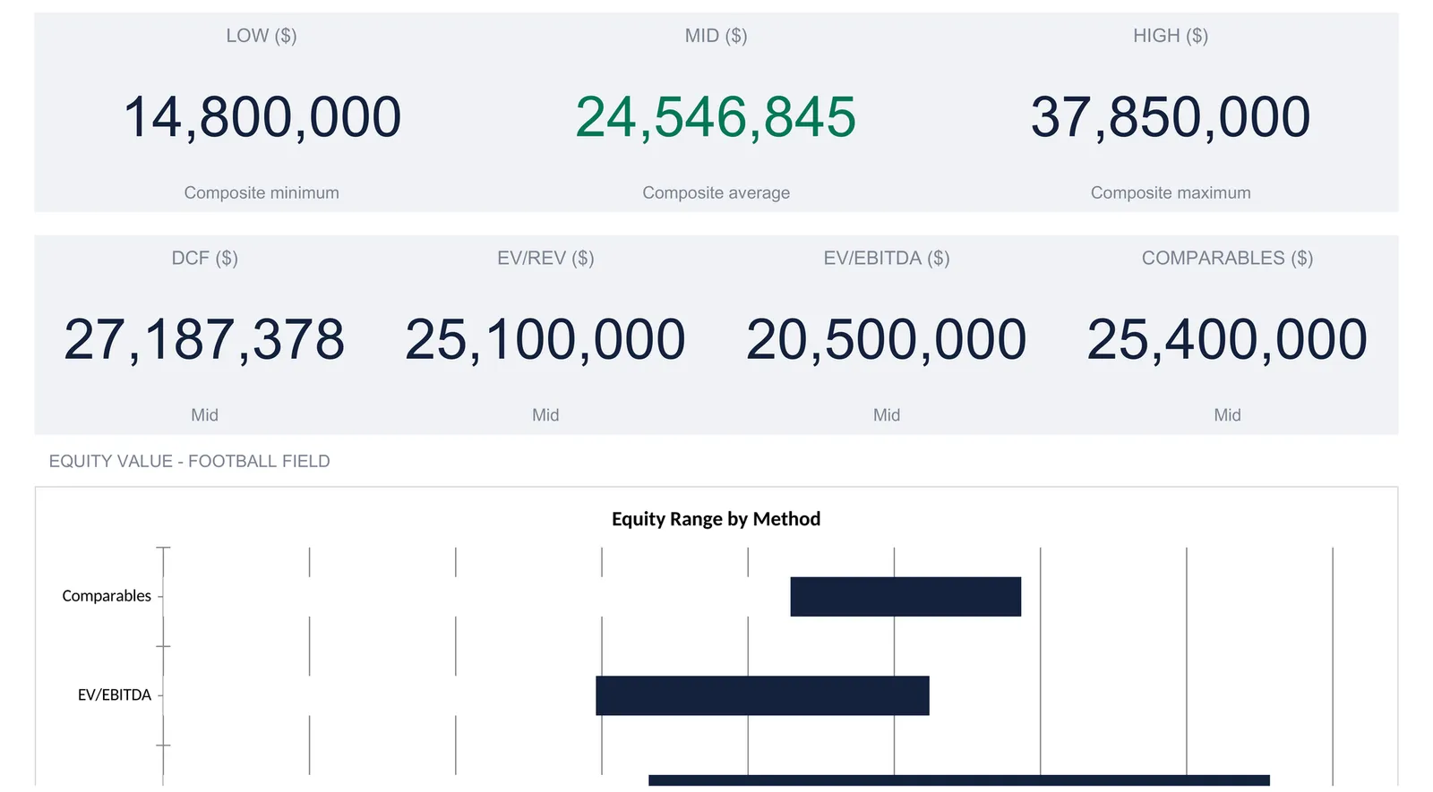
A business valuation spreadsheet runs four methods from one shared set of inputs: a 5-year discounted cash flow model, EV/Revenue and EV/EBITDA multiples, a comparable-company set, and a composite range that blends them. This walkthrough follows the full structure with a worked example, a SaaS business with $8,500,000 TTM revenue and $1,900,000 EBITDA that lands on a composite equity range of $14,800,000 to $37,850,000 with a mid near $24,500,000. Our Business Valuation Spreadsheet Template ($49) ships the same structure ready-made for Excel and Google Sheets.
Ask five people what a private company is worth and you will often get five answers, all defensible and all different. A discounted cash flow says one thing, a revenue multiple says another, and the price a similar business changed hands for last quarter says a third. None of them is wrong. Each is a different lens on the same business, and the honest answer to “what is it worth” is usually a range rather than a single number. The work of a business valuation is holding those methods next to each other and reading the spread, and a spreadsheet is a natural place to do it.
That is the structure this walkthrough follows: one set of inputs feeding four independent methods, then a composite that blends them into a low, a mid, and a high. The examples come from our Business Valuation Spreadsheet Template ($49), which ships the whole model ready-made for Excel and Google Sheets. The figures below are the workbook’s own sample, a mid-sized software business named Aurora Cloud Inc. The layout is reproducible by hand if you would rather build your own.
What a business valuation spreadsheet has to hold
Behind the jargon, a multi-method valuation needs only a few kinds of data:
- Trailing financials. What the business actually earned over the last twelve months: revenue, EBITDA, net income, and book value. Every method starts from these.
- Capital structure. Debt and cash, the two numbers that bridge the value of the business as a whole to the value that belongs to its owners.
- Assumptions. The forward-looking choices: how fast cash flow grows, what discount rate to apply, what multiples the market is paying. These are where judgment enters, and where two analysts most often disagree.
- Derived valuations. The DCF result, the multiple-based figures, the comparable-company figures, and the composite that blends them. Nothing here is typed; it all falls out of the three inputs above.
The template gives each of these its own sheet. Eight sheets in total: a Dashboard on top, then Inputs, DCF, Multiples, Comparables, and Summary, with a Settings sheet for naming and a How to Use sheet carrying the instructions. The How to Use sheet is worth a glance before starting, since it lays out the same math in one place: how the DCF grows and discounts EBITDA, how the multiples apply to the trailing figures, how the comparables take a median, and how the composite blends the four. Only two sheets take typing, Settings and Inputs; the other six are read. This walkthrough works the same way, starting with the inputs and ending at the dashboard that reads everything back.
Name the business first: the Settings sheet
The Settings sheet is deliberately small. It holds two things: the business name and a currency symbol chosen from a dropdown. In the sample they read Aurora Cloud Inc. and the dollar sign.

The name flows through to the header of every other sheet, so the workbook labels itself once. The currency symbol is a display setting: choosing one from the dropdown relabels every money column and KPI across the model. The dropdown carries more than thirty symbols, from the euro and pound to the rupee, real, and yen. Worth being clear about what this does not do. It changes the label shown next to the numbers, not the numbers themselves, so switching from the dollar to the euro does not convert anything. A note on the sheet spells this out, and it repeats a point that matters for any valuation: all of the real inputs live on the Inputs sheet, not here.
Everything the model needs: the Inputs sheet
This is the sheet that does the work of data entry. It is organized into four blocks, and once it is filled, every valuation downstream is already computed.
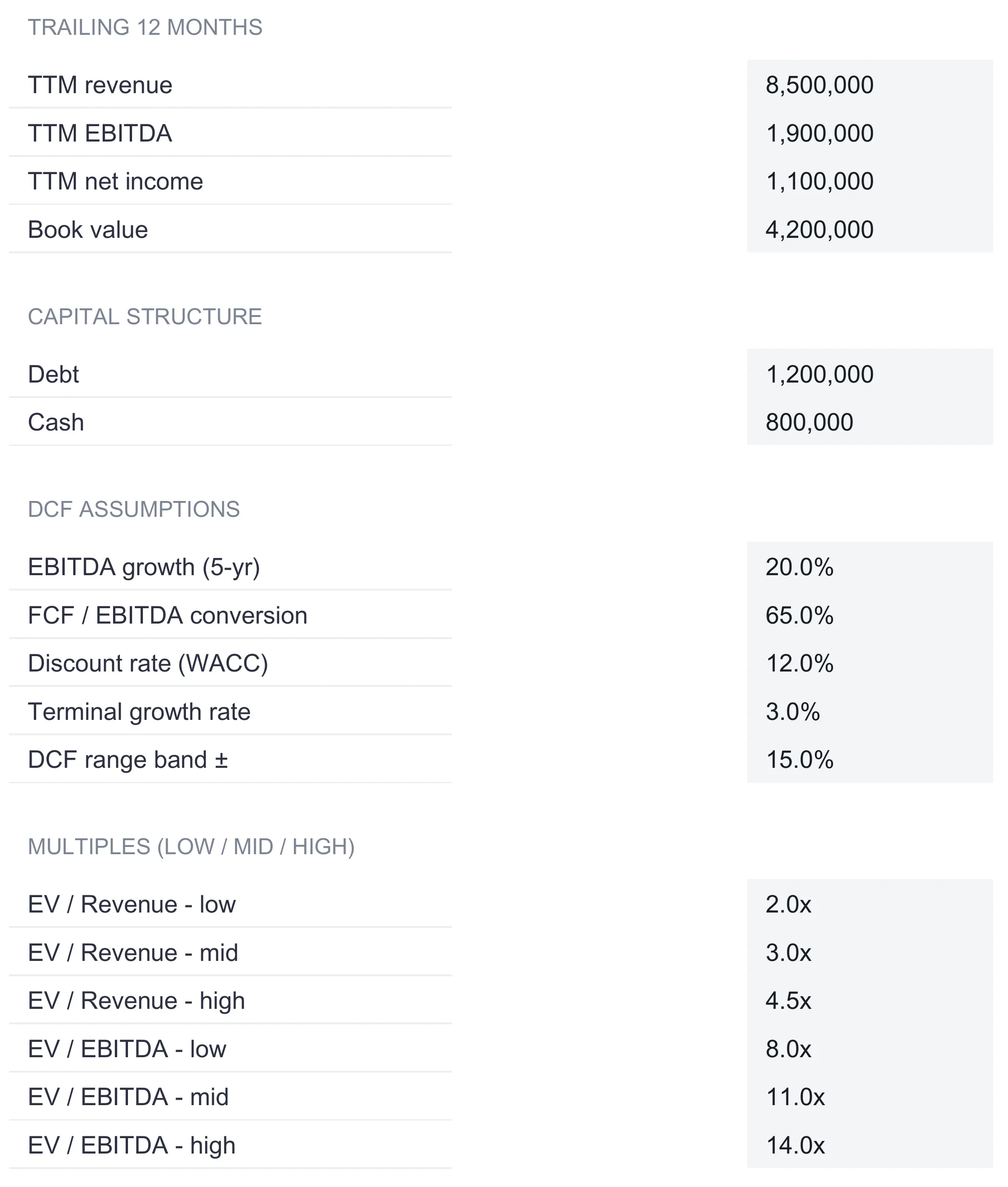
Trailing 12 months. The four figures that describe the business as it stands: TTM revenue of $8,500,000, TTM EBITDA of $1,900,000, TTM net income of $1,100,000, and book value of $4,200,000. TTM means trailing twelve months, the most recent full year of actuals rather than a calendar year. EBITDA is earnings before interest, taxes, depreciation, and amortization, a rough proxy for the cash a business generates from operations before its financing and accounting choices are layered on. Net income and book value are not used by the main methods; they feed the implied P/E and P/B cross-checks on the Summary sheet.
Capital structure. Debt of $1,200,000 and cash of $800,000. These two numbers are the bridge from enterprise value to equity value, applied identically on every method, and they are worth understanding before anything else because they explain why the dashboard’s figures differ from the raw method outputs.
DCF assumptions. Five forward-looking choices: EBITDA growth of 20.0% a year over the five-year window, an FCF-to-EBITDA conversion of 65.0%, a discount rate (WACC) of 12.0%, a terminal growth rate of 3.0%, and a DCF range band of plus or minus 15.0%. The band is a nice touch: the DCF produces a single point estimate, and the band is what turns that one number into a low and a high on the Summary.
Multiples. Six numbers in a low, mid, high grid: EV/Revenue at 2.0x, 3.0x, and 4.5x, and EV/EBITDA at 8.0x, 11.0x, and 14.0x. These are the market multiples the model applies to the trailing figures, and they are the single most subjective input in any relative valuation.
A note at the foot of the sheet restates the identity that runs through the whole workbook: equity value equals enterprise value minus debt plus cash. Everything else is arithmetic on top of that.
Method one: the DCF sheet
The first method is a five-year discounted cash flow. In plain terms, a DCF estimates what a business is worth today by projecting the cash it will throw off in future years and discounting each year back to a present value, on the principle that a dollar arriving in year five is worth less than a dollar in hand now.
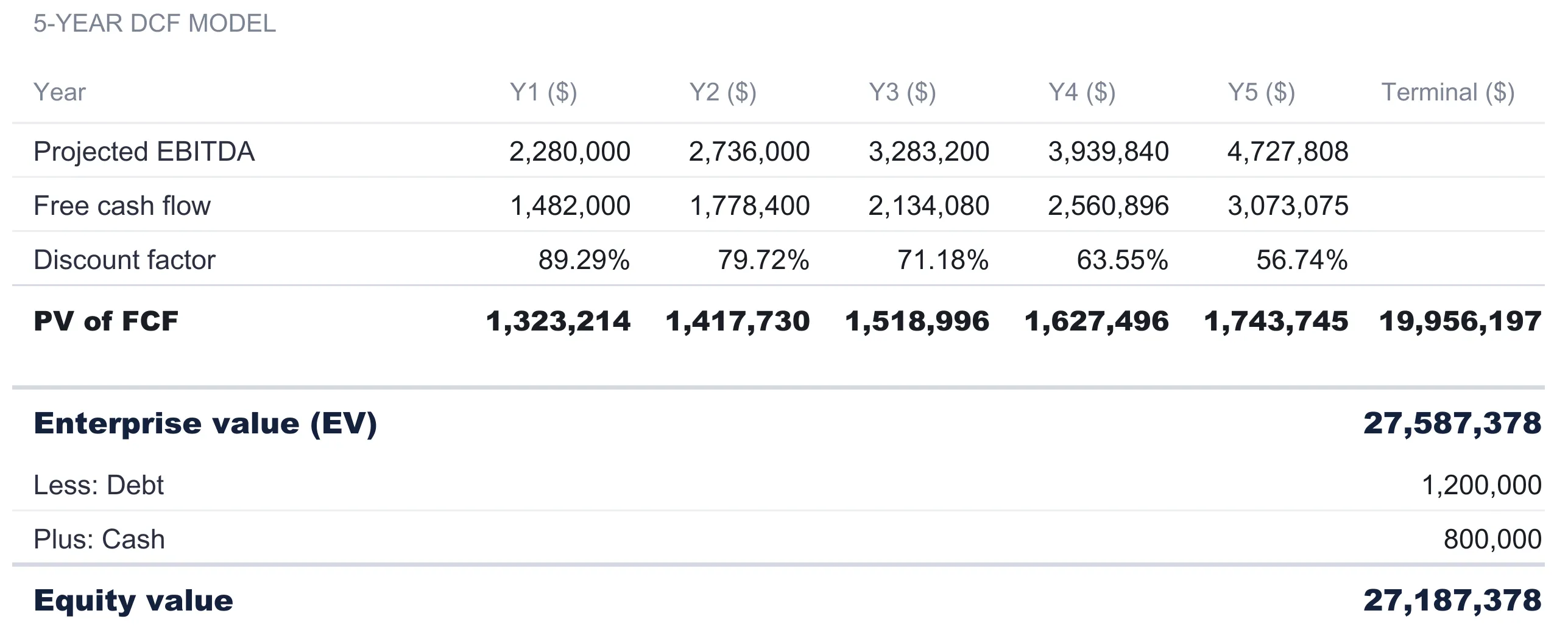
The sheet builds up in layers, one row at a time, across years Y1 through Y5 plus a terminal column:
- Projected EBITDA grows the $1,900,000 starting EBITDA at 20.0% a year: $2,280,000 in Y1, then $2,736,000, $3,283,200, $3,939,840, and $4,727,808 by Y5.
- Free cash flow takes 65.0% of each year’s EBITDA, the conversion assumption from Inputs. Y1 lands at $1,482,000 and Y5 at $3,073,075.
- Discount factor is one divided by (1 plus WACC) raised to the year number. At a 12.0% WACC it falls from 89.29% in Y1 to 56.74% in Y5, the mathematical statement that later cash is worth less today.
- PV of FCF multiplies each year’s free cash flow by its discount factor: $1,323,214 in Y1 down through $1,743,745 in Y5.
The terminal column is where most of the value sits, and it is worth slowing down on. A five-year projection has to say something about everything after year five, and this model uses the stable-growth approach. It assumes free cash flow grows at the 3.0% terminal rate forever and capitalizes it with the Gordon-growth formula: year-five cash flow times (1 plus g), divided by (WACC minus g). That figure is then discounted back five years. In the sample the discounted terminal value is $19,956,197, comfortably the largest single piece. That concentration is normal for a growing business and is exactly why the terminal assumptions deserve scrutiny; the NYU Stern note on estimating terminal value walks through why the stable-growth version is the one that stays consistent with the rest of a DCF.
The formula carries a guard. Because the divisor is WACC minus growth, the terminal value would break if the discount rate were at or below the terminal growth rate, so the sheet returns zero in that case rather than a meaningless figure. The discount factors carry a similar guard against a WACC that is not above negative one hundred percent. Neither trips in the sample, but they are the kind of defensive wiring that keeps a model from silently producing nonsense when someone stress-tests an assumption.
Summing the five present values and the discounted terminal value gives an enterprise value of $27,587,378. The sheet then applies the bridge, subtracting the $1,200,000 of debt and adding the $800,000 of cash, to reach an equity value of $27,187,378. That is the DCF’s single answer.
Methods two and three: the Multiples sheet
Where the DCF looks forward, a multiples valuation looks sideways, at what the market pays for a dollar of revenue or a dollar of EBITDA. The Multiples sheet runs two of them, each in a low, mid, high grid, so a single price never has to carry the whole judgment.
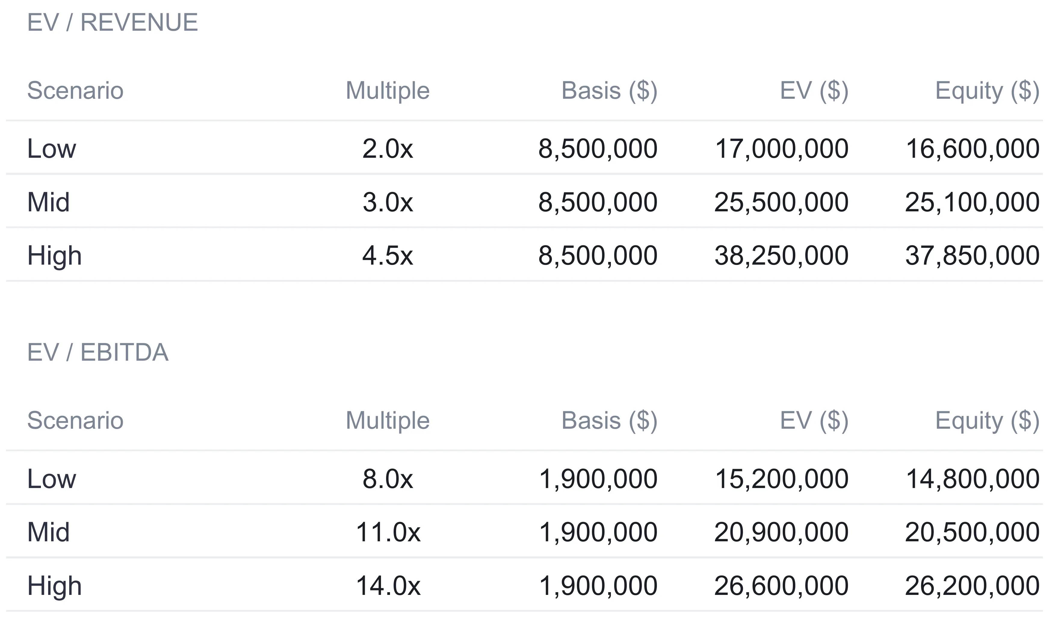
The mechanics are the same in both tables: multiply the trailing-12-month basis by the chosen multiple to get an enterprise value, then apply the debt-and-cash bridge to reach equity.
EV/Revenue applies the 2.0x, 3.0x, and 4.5x multiples to the $8,500,000 revenue basis. That produces enterprise values of $17,000,000, $25,500,000, and $38,250,000, which become equity values of $16,600,000, $25,100,000, and $37,850,000 after the bridge.
EV/EBITDA applies the 8.0x, 11.0x, and 14.0x multiples to the $1,900,000 EBITDA basis, for enterprise values of $15,200,000, $20,900,000, and $26,600,000, and equity values of $14,800,000, $20,500,000, and $26,200,000.
Two things stand out. The revenue method lands higher than the EBITDA method at every tier, which is typical of a business whose margins are thinner than the multiples imply, and it is one reason a valuation shows both rather than trusting either alone. The CFA Institute’s reference on price and enterprise value multiples is a good grounding in why EV/EBITDA in particular is often preferred for comparing businesses with different debt loads, since EBITDA sits above interest in the income statement. The other point is practical: because these figures read straight from the Inputs multiples, editing the six numbers on the Inputs sheet reprices both tables at once.
Method four: the Comparables sheet
The comparables method answers a different question again: what are similar businesses actually trading at? Rather than choosing multiples in the abstract, it derives them from a peer set.
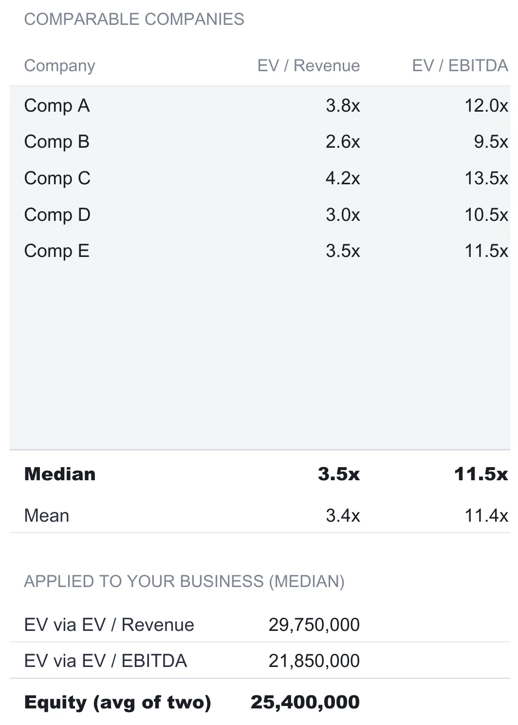
The sample ships five comparable companies, Comp A through Comp E, each with its own EV/Revenue and EV/EBITDA multiple. The sheet then takes the median of each column, 3.5x on revenue and 11.5x on EBITDA, and it is the median, not the mean, that drives the result. The mean is shown alongside for reference at 3.4x and 11.4x, but it feeds nothing. Median is the more robust choice here because a single outlier comp, a Comp C trading at 4.2x revenue, pulls a mean around without much changing a median.
The applied block puts those medians to work on the business itself. The revenue median gives an enterprise value of $29,750,000 (3.5x times $8,500,000), the EBITDA median gives $21,850,000 (11.5x times $1,900,000), and the equity figure of $25,400,000 averages those two enterprise values and then applies the debt-and-cash bridge.
It is worth being clear about how this method differs from the Multiples sheet, since both traffic in EV/Revenue and EV/EBITDA. The Multiples sheet applies numbers the analyst chooses, a deliberate low, mid, and high scenario. The Comparables sheet instead reads those multiples off a real peer group and lets the median settle the figure, which grounds the valuation in observed prices rather than a view. Running both is not redundant; it checks a chosen multiple against what the market is paying, and the two landing close together is itself a signal that the assumptions are reasonable.
One design detail is worth copying into any hand-built version. Below the five filled comps sit five spare rows, and they are already inside the median and mean formulas. Typing a real peer into a spare row folds it straight into the calculation, because MEDIAN and AVERAGE both skip blank rows and both work in Excel and Google Sheets without any add-on. There is no range to extend and no formula to drag, which is the same wiring habit that keeps the rest of the workbook from drifting as it fills.
Bringing it together: the Summary sheet
Four methods have now produced their own view. The Summary sheet is where they are laid out together and blended, and it is the sheet the dashboard reads from.
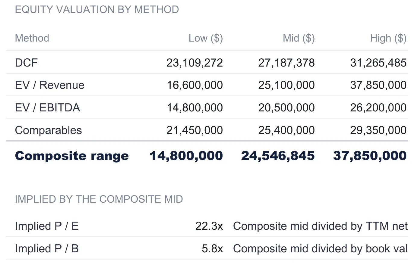
Each method gets a low, mid, and high row:
- DCF shows $23,109,272, $27,187,378, and $31,265,485. The mid is the DCF’s single answer from earlier; the low and high are that number flexed down and up by the 15.0% DCF range band from Inputs. This is where the band earns its place, turning one point estimate into a range without a second model.
- EV/Revenue carries its own $16,600,000, $25,100,000, and $37,850,000 straight from the Multiples sheet.
- EV/EBITDA carries $14,800,000, $20,500,000, and $26,200,000.
- Comparables shows $21,450,000, $25,400,000, and $29,350,000, where the low and high are the lower and higher of the two median-based enterprise values bridged to equity, and the mid is their average.
The composite range at the foot blends the four in a deliberately asymmetric way: the minimum of all the lows, the average of the mids, and the maximum of the highs. That gives $14,800,000, $24,546,845, and $37,850,000. The composite low is the EV/EBITDA low and the composite high is the EV/Revenue high, because the composite reaches for the widest defensible span rather than averaging the extremes away. The mid, by contrast, is a straight average of the four method mids, which keeps it centered.
Below the composite sit two cross-checks. The implied P/E of 22.3x divides the composite mid by the $1,100,000 TTM net income, and the implied P/B of 5.8x divides it by the $4,200,000 book value. These are sanity checks rather than valuation methods: they translate the composite into the price-to-earnings and price-to-book language an investor recognizes, so an obviously implausible multiple would flag a bad assumption upstream. They read nothing else in the model, and each goes blank if the figure it divides by is not above zero.
The dashboard: one range, four methods, one chart
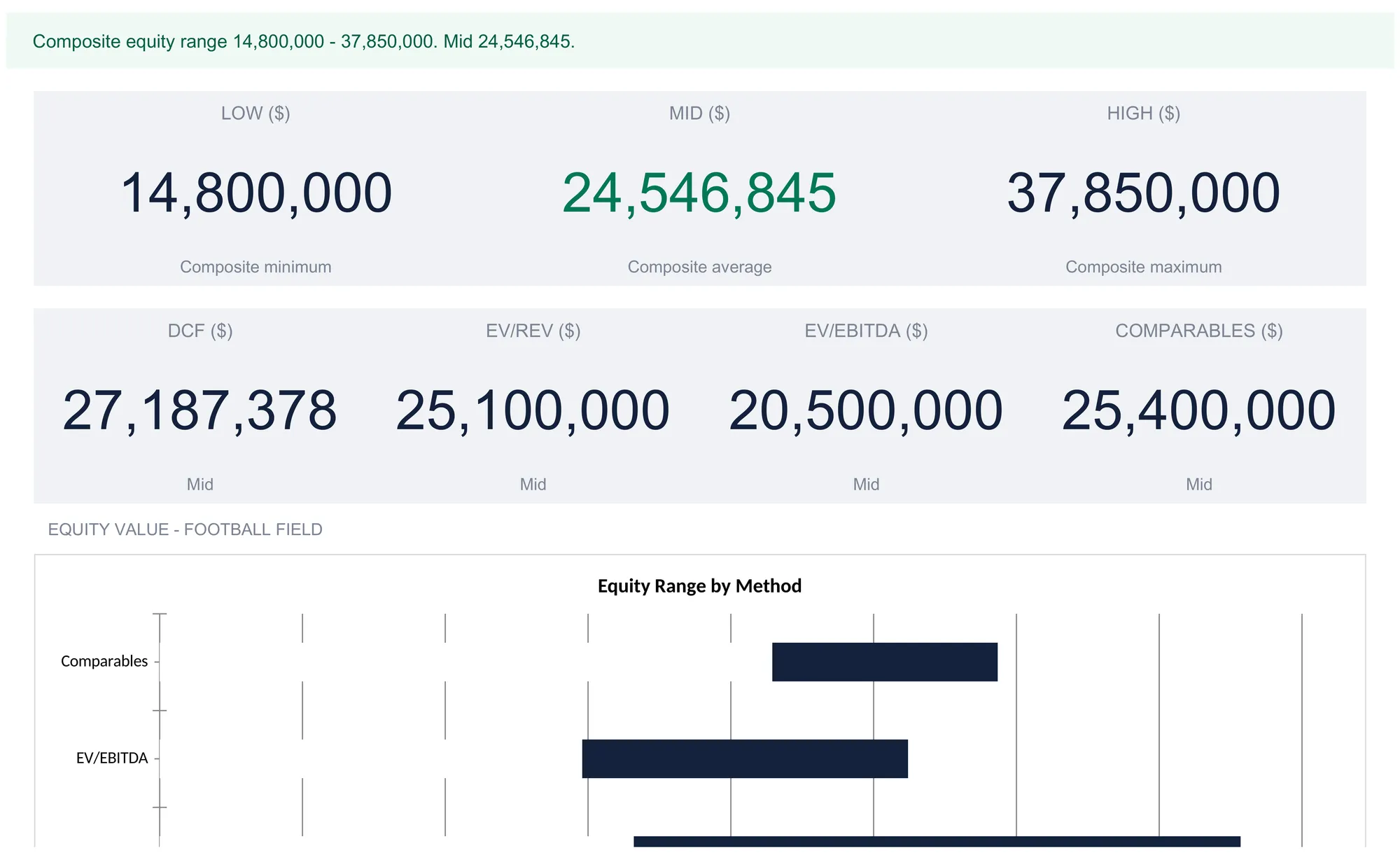
With the three input sheets filled, the Dashboard reads the whole valuation back in a form built to be understood at a glance. It opens with a status line stating the composite equity range in one sentence, then three large tiles for the composite low, mid, and high: $14,800,000, $24,546,845, and $37,850,000. Below those, four smaller tiles give each method’s mid side by side, $27,187,378 for the DCF, $25,100,000 for EV/Revenue, $20,500,000 for EV/EBITDA, and $25,400,000 for Comparables, so the spread between approaches is visible without opening another sheet.
The dashboard’s centerpiece is a football-field chart, the standard way valuation work is presented: one horizontal bar per method, each spanning from its low to its high, so the eye reads both the center and the width of every method at once. A method with a tight bar is one whose assumptions leave little room; a wide bar signals a method that is sensitive to its inputs. Reading the four bars together is the point of running four methods, and it is why the output of this model is a picture of a range rather than a single headline number.
The composite mid of roughly $24,500,000 is the number most people will quote, but the honest takeaway sits in the span around it. A business that a DCF values near $27,000,000 and an EBITDA multiple values near $20,500,000 is not worth precisely either figure; it is worth an amount that depends on which lens a buyer trusts, and seeing all of them on one screen is most of the reason to build the model at all.
Enterprise value, EBITDA, WACC, and terminal value in plain terms
Four pieces of jargon do most of the heavy lifting in this workbook, and none of them is complicated once unpacked.
Enterprise value is the value of the entire business to everyone who funded it, lenders and owners together. Equity value is what remains for the owners after the debt is cleared and the cash is counted, which is why every method here computes equity as enterprise value minus the $1,200,000 debt plus the $800,000 cash.
EBITDA is earnings before interest, taxes, depreciation, and amortization. Stripping those four out gives a rough, financing-neutral view of operating cash generation, which is what makes it a common basis for comparing businesses that carry different debt and tax situations.
WACC, the weighted average cost of capital, is the discount rate a DCF uses to pull future cash back to the present. A higher WACC means future cash is discounted harder and the business is worth less today. The sample uses 12.0%.
Terminal value is the catch-all for every cash flow beyond the explicit five-year window, capitalized with the Gordon-growth formula and then discounted back. Because it stands in for an infinite tail, it usually dominates a DCF, as the $19,956,197 in the sample does, and it is the assumption most worth pressure-testing.
Excel or Google Sheets for a business valuation
The template is an .xlsx file built on plain formulas, with no macros and no add-ons, so it behaves identically in Microsoft Excel and in Google Sheets after an upload. The functions the model leans on, MEDIAN and AVERAGE on the Comparables sheet and the power and IF logic behind the DCF, are native to both platforms. Excel suits anyone who prefers a local file and heavy keyboard work; Google Sheets suits collaborators who want to comment on assumptions in a shared link. The structure described here builds the same way in either, and the same spreadsheet template runs in both without a change.
Which template fits the job
- Business Valuation Spreadsheet Template ($49) is the workbook this walkthrough follows: the shared Inputs sheet, the five-year DCF, the EV/Revenue and EV/EBITDA multiples, the comparable-company set, and the composite range and dashboard that read them all back. It suits anyone valuing a single going-concern business from its trailing financials.
- 5-Year Financial Projections Spreadsheet Template ($49) sits on the other side of the same question. Where the valuation model takes trailing financials as a given and prices them, the projections model is where those forward numbers get built in the first place, a three-statement forecast that produces the revenue and cash flow a DCF ultimately relies on. Owners preparing for a raise or a sale often work through the projections first and the valuation second.
Both are part of the same business-planning family, and a founder assembling a full package tends to reach for the pair together.
Related
- How to Build a Startup Financial Model in a Spreadsheet - burn, runway, and the cap table behind an early-stage raise
- How to Build 5-Year Financial Projections in a Spreadsheet - the three-statement projection that feeds a DCF
- How to Analyze a Rental Property in a Spreadsheet - NOI, DSCR, and cash-on-cash for a property purchase
Frequently asked questions
What is the difference between enterprise value and equity value?
Enterprise value is what the whole business is worth to all providers of capital, before its own balance sheet is taken into account. Equity value is what is left for the owners once debt is repaid and cash on hand is added back. The template computes equity as enterprise value minus debt plus cash on every method, using the $1,200,000 debt and $800,000 cash from the Inputs sheet, so the low, mid, and high figures on the Summary are all equity values that an owner can read directly.
Why do the DCF, multiples, and comparables give different valuations?
Each method looks at the business through a different lens. The DCF discounts projected cash flows, the revenue and EBITDA multiples price the trailing 12 months against chosen market multiples, and the comparables apply the median multiple of a peer set. In the sample they land between a $20,500,000 EV/EBITDA mid and a $27,187,378 DCF mid. The Summary keeps all four side by side rather than picking a winner, and its composite takes the minimum of the lows, the average of the mids, and the maximum of the highs.
What happens if the discount rate is at or below the terminal growth rate?
The terminal value reads zero. The Gordon-growth formula the model uses divides by the discount rate minus the growth rate, which is undefined when the two are equal and negative when growth is higher, so the sheet carries a guard that returns zero rather than a nonsense number. The sample keeps a 12.0% WACC well above the 3.0% terminal growth rate, so the terminal value contributes its full $19,956,197 of present value.
Can I replace the sample comparable companies with my own?
Yes. The Comparables sheet ships five filled rows, Comp A through Comp E, plus five spare rows below them. Typing a company and its EV/Revenue and EV/EBITDA multiples into a spare row adds it to the median and mean, and the applied enterprise values below recalculate automatically because they read the median. The MEDIAN and AVERAGE functions skip blank rows, so unused spares do not distort the result.
Does the currency selector convert the numbers or just relabel them?
It relabels only. The Settings sheet holds a business name and a currency symbol chosen from a dropdown, and picking a symbol updates every column header and KPI label across the workbook. It changes the label shown next to the figures, not the figures themselves, so the underlying amounts stay exactly as entered.
Sources
- Estimating Terminal Value - Aswath Damodaran, NYU Stern School of Business
- Market-Based Valuation: Price and Enterprise Value Multiples - CFA Institute
About this article
Every figure, column name, formula, and feature description verified against the published Business Valuation Pro workbook (the exact file customers download). Terminal value and market-multiple references checked against the live NYU Stern and CFA Institute pages at writing time. Last reviewed August 2026.