
Track multiple savings goals in Google Sheets with the bucket-allocation method: one savings account, many named buckets in the sheet. Give each goal five columns (target, due date, monthly contribution, current balance, percent complete), add one reconciliation row that ties the buckets back to the bank balance, and a single progress chart. Most people run three to six goals comfortably this way.
Running one savings goal is easy. Running five at once, covering a house down payment, a replacement car, a trip, a wedding and a laptop, is where the spreadsheet stops being a luxury and starts being the only thing holding the plan together. A single savings account balance does not tell you whether the down payment is on track or whether the trip fund has already been quietly raided. This guide builds the structure by hand; our free Savings Goal Tracker ships the goal rows ready to use, with target, saved, remaining and target-date columns, and the Annual Budgeting Planner tracks year-end goals next to a 12-month plan-and-actual budget.
Why multi-goal tracking falls apart
A few patterns show up in setups that don’t survive past three months.
One balance, many goals. The account shows $7,400. Three goals are supposed to live inside it. Which one took the hit when $400 left last week? Without a tracker, the smallest goal absorbs every overrun.
No contribution math. Picking “$5,000 for the trip in 10 months” without dividing by 10 leaves the monthly number invisible. The first few months go fine on momentum; by month four the gap is real.
Too many goals. Above eight active goals, contributions shrink to amounts where progress feels like noise. People abandon goals when the bar moves a millimeter at a time.
No honest record when a goal slips. A trip gets cancelled, a car repair eats the emergency fund, the down payment gets pushed out a year. If those events don’t get logged, the tracker drifts and stops being trusted.
The fixes are structural, not motivational.
The bucket-allocation method
The core idea: one bank account holds the money, but a spreadsheet tracks how that single balance is divided across named buckets. Each bucket has its own target, deadline, and progress. The allocation is virtual, so nothing moves at the bank when a bucket changes.
| Goal | Allocated | Held in |
|---|---|---|
| House down payment | $12,500 | Main HYSA |
| Replacement car | $4,200 | Main HYSA |
| Italy trip | $1,800 | Main HYSA |
| Wedding | $5,000 | Joint HYSA |
| Laptop | $1,320 | Main HYSA |
| Total | $24,820 |
The “held in” column matters once the money stops living in one place, which happens more often than people expect: a joint account for the shared goal, an old account nobody got around to closing. Four buckets above add up to $19,820 in the main account and one holds $5,000 in the joint account.
The invariant that keeps the system honest:
Account balance = Sum of the "current balance" cells for buckets held thereWhen the two sides disagree, something has not been recorded. Catching it at $15 is easy. Catching it at $1,200 takes an afternoon.
This is the same allocation idea behind sinking funds, but applied to discrete targets rather than recurring expenses. Sinking funds reset every year (the December insurance bill comes back). Savings goals usually end (the down payment closes, the trip happens, the car gets bought).
The five-column layout
Five columns per goal cover everything material. Anything else is decoration.
| Goal | Target | Due date | Monthly contribution | Current balance | Percent complete |
|---|---|---|---|---|---|
| House down payment | $40,000 | 2028-07-01 | $1,250 | $12,500 | 31% |
| Replacement car | $18,000 | 2027-09-01 | $1,150 | $4,200 | 23% |
| Italy trip | $6,000 | 2027-05-01 | $525 | $1,800 | 30% |
| Wedding | $22,500 | 2027-10-15 | $1,347 | $5,000 | 22% |
| Laptop | $2,200 | 2026-11-01 | $440 | $1,320 | 60% |
| Total | $88,700 | $4,712 | $24,820 | 28% |
The contribution column above is calculated as of August 2026, so it climbs a little every month a deadline gets closer without the balance moving.
Target is the dollar amount you decided this goal needs. Round numbers are fine.
Due date is when the money has to be there. Some goals are firm (closing date, trip departure); others are flexible (laptop replacement). Use a real date either way - the math depends on it.
Monthly contribution is calculated, not chosen. The formula:
=ROUNDUP((B2 - E2) / DATEDIF(TODAY(), C2, "M"), 0)That is (target minus current balance) divided by months remaining, rounded up so you arrive a little early rather than $13 short. DATEDIF returns full months between today and the due date.
Current balance is what is actually in this bucket. Either you update it monthly by adding the contribution and subtracting any withdrawals, or you let a contribution log fill it in for you, which the section below covers.
Percent complete is current balance / target formatted as a percentage. The visible progress number is what keeps people coming back.
The six formulas that run the sheet
Everything else on the sheet derives from those columns. Written against row 2 of the table above, where column A is the goal name and column F is percent complete:
Remaining          =B2-E2
Percent complete   =E2/B2
Overall progress   =SUM(E2:E6)/SUM(B2:B6)
Months at this pace =IF(D2>0,ROUNDUP((B2-E2)/D2,0),"")
Required monthly   =IFERROR(ROUNDUP((B2-E2)/DATEDIF(TODAY(),C2,"M"),0),B2-E2)
On track?          =IFERROR(IF(E2>=B2-D2*DATEDIF(TODAY(),C2,"M"),"On track","Behind"),"Past due")
Two of those need a word of explanation. The required-monthly formula divides by months remaining, which hits zero in the goal’s final month, so the IFERROR wrapper falls back to the whole remaining amount rather than showing #DIV/0!. The on-track check works backwards from the deadline: it asks whether the balance today is already high enough that the planned contribution in column D still lands on target. Every row in the sample table reads “On track” because the contributions were derived from those balances in the first place; the column earns its keep in month three, once real deposits have diverged from the plan.
Overall progress across the five goals comes out at $24,820 against $88,700, or 28 percent. That single number is the one worth putting somewhere visible.
The monthly routine
Five minutes per month, on a fixed day. Payday or the statement date both work.
- Open the bank account, note the actual balance.
- For each goal row, add the contribution to current balance. Subtract anything spent from that bucket.
- Sum the current-balance column. Compare to the bank balance.
- If they match within a few dollars (interest, rounding), close the sheet.
- If they don’t, find the missing transaction before doing anything else.
Step 5 is the one that gets skipped. Drift wins if it gets skipped twice in a row.
The contribution log
Step 2 above is the weak point, because a hand-edited balance keeps no history. A second sheet named Log fixes that: date in column A, goal name in column B, amount in column C, one row per movement.
| Date | Goal | Amount |
|---|---|---|
| 2026-08-01 | House down payment | $1,250 |
| 2026-08-01 | Wedding | $1,347 |
| 2026-08-01 | Replacement car | $1,150 |
| 2026-08-14 | Italy trip | -$400 |
Withdrawals go in as negative amounts, which is what lets one formula handle both directions. The current-balance column on the main sheet then stops being typed and becomes a SUMIF:
=SUMIF(Log!$B:$B, A2, Log!$C:$C)Because the goal name in A2 is the lookup key, a typo in the log silently drops that row from the total. Making column B of the log a dropdown, using Data > Data validation pointed at the goal-name column, removes that failure mode.
The trade-off is honest: the log costs one extra row per deposit and gives back a full history, a balance that cannot be fudged, and a variance check. Comparing what a goal actually received this month against column D shows which buckets are quietly running behind before the deadline does.
The reconciliation row
A single formula at the bottom of the sheet makes the invariant visible:
=ABS(SUM(E2:E10) - H1)Where H1 sits just outside the table and holds the actual bank balance, retyped each month. Wrap the result in conditional formatting so it turns red over a $5 threshold. Now the spreadsheet tells you when it has drifted from reality, instead of waiting for you to notice.
The progress view
Two visualizations carry their weight; everything beyond that is clutter.
A horizontal bar per goal. One row, one bar, one number, read in a second. Three ways to draw it, in rough order of how much they cost to set up.
SPARKLINE puts a real bar inside a cell next to the percentage:
=SPARKLINE(F2,{"charttype","bar";"max",1;"color1","#188038"})A color scale on the percent-complete column takes no formula at all. Format > Conditional formatting > Color scale, with the minpoint at 0 and the maxpoint at 1, gives the same read at a glance.
A text bar built from REPT survives being copied into a plain-text note or a message to a partner, which the other two do not:
=REPT("█",ROUND(MIN(F2,1)*10,0))&REPT("░",10-ROUND(MIN(F2,1)*10,0))At 31 percent that renders ███░░░░░░░. The MIN is load-bearing: without it, a bucket that overshoots its target pushes the second REPT to a negative count and the cell breaks with an error on exactly the goal that went well.
A stacked bar showing the bucket split across the total balance. Insert > Chart, stacked bar, one bar with one segment per goal. The chart that answers “where does the $24,820 actually live.”
A line chart over time is tempting and rarely worth the maintenance. The percent-complete column already tells the same story.
Picking the monthly contribution when reality pushes back
The formula gives you a number. The household budget gives you a different number. When the five goals above ask for $4,712 a month and the budget can spare $1,800, three options come up.
Stretch the timeline. Push the due date out until the contribution fits. Moving the down payment from July 2028 to July 2029 takes it from 22 months of runway to 34, and the monthly number falls from $1,250 to $809.
Shrink the target. A $40,000 down payment becomes a $28,000 down payment at a different price point or with a different loan structure. The target was an input, not a law.
Sequence the goals. Pause one bucket while another fills. The house fund can sit at $0 for six months while the laptop and trip buckets clear their nearer deadlines, at the cost of $27,500 then needing to arrive in 16 months instead of 22.
In practice most multi-goal setups settle into some mix of all three. Naming the trade-off is the value the spreadsheet adds; a single savings balance hides it.
Splitting a fixed monthly amount across buckets
The section above works backwards from targets. Plenty of people work forwards instead: a fixed amount lands in savings every month and the question is how to divide it. Three methods show up, and the sheet handles all three the same way, by feeding column D.
Fixed amounts. Type a number into column D for each goal and leave it. Simple, stable, and it stops reflecting reality the moment income or a deadline changes.
Percentages of the pot. Each goal gets a share, and the dollar amounts recalculate on their own when the pot moves.
| Goal | Share | Of $1,800 |
|---|---|---|
| House down payment | 40% | $720 |
| Wedding | 25% | $450 |
| Replacement car | 20% | $360 |
| Italy trip | 10% | $180 |
| Laptop | 5% | $90 |
A waterfall. Goals fill in row order, each taking what it needs until the pot runs out. With the monthly pot in H2 and allocations in column G, one formula fills down the whole column:
=MAX(0, MIN($H$2 - SUM($G$1:G1), D2, B2-E2))SUM($G$1:G1) is what earlier rows have already claimed, and it expands as the formula fills down. The three arguments inside MIN are the three ceilings that matter: what is left in the pot, the planned monthly contribution, and the amount still needed to finish the goal. Dropping the last two is the version that goes wrong, because the first row then swallows the entire pot every month.
On the $1,800 pot, the row order above gives the house its full $1,250, hands the remaining $550 to the car, and leaves the trip, wedding and laptop at zero. That is the waterfall being honest rather than broken. Reordering the rows changes who gets funded, which is the whole point of the method and also its main risk: the laptop has the nearest deadline of the five and sits last in line.
Months rarely come out even. When the deposit falls short, some sheets scale every bucket down by the same ratio and others simply skip the bottom rows; when a windfall lands, the same choice runs in reverse. Either way the contribution log records what actually happened, so the on-track column picks up the difference without anyone having to remember it.
When a goal slips
Goals miss their dates. The trip gets cancelled, the car holds together another year, the wedding venue moves a quarter. Three approaches keep the tracker honest:
Edit in place. Change the due date or the target, let the formula recalculate the monthly contribution. Note the change in a comments column so the history is visible.
Close the bucket, move the money. If the goal is genuinely cancelled, transfer the balance to another bucket and mark the row complete. A tracker that still shows a dead goal eventually stops being trusted.
Log a withdrawal. If life pulled money out of a goal early, subtract it from current balance the day it happens. A bucket whose target says $6,000 and current balance says $1,800 after a withdrawal tells you the truth. A bucket that still says $3,200 because you didn’t update it lies.
The option that breaks the system long-term is the quiet one, where a goal gets abandoned and the spreadsheet is never told.
How many goals is workable
Most multi-goal trackers stabilize at three to six active goals. Above eight, contributions get so small that progress disappears into the noise of normal account movement.
Two ways to compress:
Combine related buckets. “Trip” instead of “Italy 2027” plus “Iceland 2028” plus “Mexico 2028” - one bucket, one larger target, one progress bar. The detail can live in a notes column.
Hold goals as queued, not active. Goals that exist but aren’t getting contributions sit in a separate sheet with a target and a due date but no monthly number. They are real plans without crowding the active view.
Our free Savings Goal Tracker tracks up to seven goals with target, saved, remaining and target-date columns plus an at-a-glance total, if rebuilding it from scratch sounds like more work than it’s worth. A step-by-step build, formula by formula, is in How to Build a Savings Goal Tracker in Google Sheets.
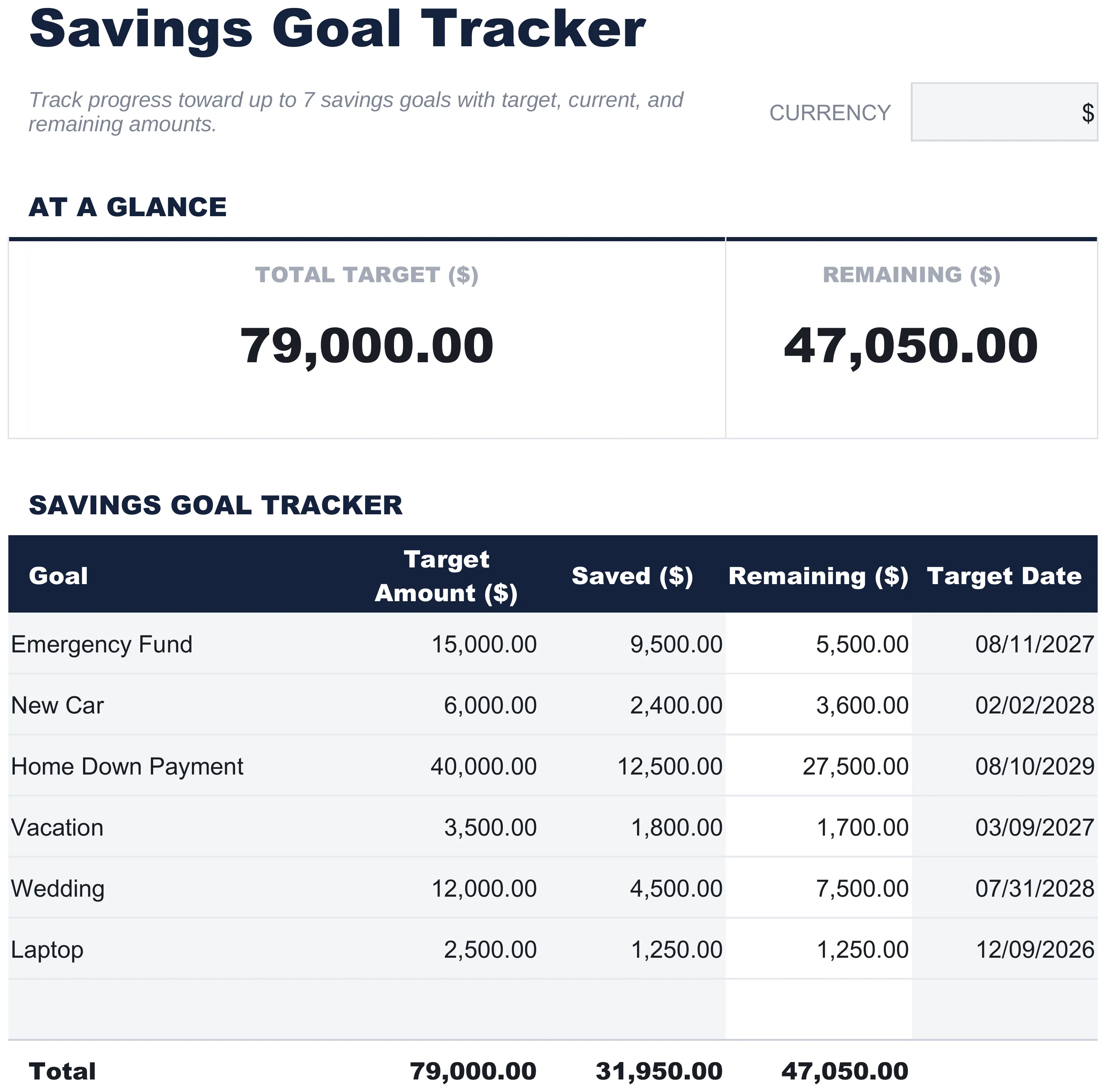 The free Savings Goal Tracker template (Free tier) tracks up to seven goals with an at-a-glance total and a currency selector.
Bank features that replicate this
Some banks offer the bucket structure natively. The relevant feature names as of 2026:
| Bank | Feature | Notes |
|---|---|---|
| Ally | Savings Buckets | Up to 30 named buckets inside one Online Savings account, no extra fees |
| Capital One | Multiple 360 Performance Savings accounts | Open separate accounts per goal, named individually, no fees or minimums |
| SoFi | Vaults | Up to 20 vaults inside one Savings account |
| Marcus by Goldman Sachs | Multiple savings accounts | Open up to a small number per customer with separate nicknames |
The bank version answers “where does each dollar belong” in their UI, so a spreadsheet becomes optional. Trade-offs: rebalancing buckets takes more clicks than editing two cells, projecting monthly contributions requires their UI or no UI at all, and switching banks means rebuilding the whole structure.
For yield context, the FDIC national average savings rate sat at 0.38 percent as of August 2026, while online high-yield savings accounts commonly pay 4 to 5 percent APY. On the kind of balances multi-goal trackers hold, the rate matters more than the UI features.
When the free tracker isn’t enough
A spreadsheet built from the columns above handles three to six goals with a five-minute monthly routine. Its limits show up at the edges:
- More than eight active goals where the layout starts feeling cramped.
- Goals that interact with the household budget, so contributions belong alongside actual expense tracking.
- A partner who would rather not learn the formulas.
These are the cases a built template earns its keep over a blank sheet.
Templates that fit this
- “I just want multiple goals tracked, free.” Savings Goal Tracker. Up to seven goals with target, saved, remaining and target-date columns, an at-a-glance total-and-remaining summary, and a currency selector. The bucket idea, already wired up.
- “I want goals inside a full year-long budget.” Annual Budgeting Planner at $29 once. A 12-month plan-and-actual grid for income, expenses and savings, plus an Annual Financial Goals sheet where every goal carries a target, a starting balance and the monthly amount required to reach it by December 31.
The free tracker opens in Google Sheets, Microsoft Excel, or LibreOffice Calc, with no macros and no data collection. The Annual Budgeting Planner is a Google Sheets template.
Related
Frequently asked questions
How many goals is too many?
Most people manage 3 to 6 active goals well. Above 8, contribution amounts become so small that progress feels invisible and goals get abandoned. Combining smaller goals into broader buckets is a common fix.
Should every goal have its own savings account?
No. One account with a spreadsheet that tracks allocations works for most people. Some banks offer 'sub-accounts' or buckets that let you do this without a spreadsheet, but the math is the same.
What is the bucket-allocation method?
Each savings goal is a 'bucket' that the spreadsheet tracks separately, even when all goals share one bank account. Monthly contributions go into specific buckets. The bank balance matches the sum of all buckets.
What if I have to dip into one goal?
Mark it in the spreadsheet. The honest record matters more than hitting the original target. Adjust the contribution schedule going forward or extend the timeline.
What happens when a goal is fully funded?
The row usually stays until the money is actually spent, then comes out. Some trackers keep a completed section below the active rows so the history stays visible; others move the row to a second sheet. Leaving a funded goal in the active list with a contribution still assigned to it is what pushes the reconciliation row out of balance.
Does this work in Excel?
The layout does, and so do most of the formulas. DATEDIF, SUMIF, REPT and ROUNDUP all exist in Excel. SPARKLINE does not: Excel covers the same in-cell progress bar with data bars under conditional formatting.
Should retirement be one of the goals?
Most multi-goal trackers leave it out. Retirement accounts carry employer contributions, their own tax treatment and a horizon measured in decades, so they behave differently from a bucket with a due date. They tend to show up in net worth tracking instead.
Where does the interest go when several goals share one account?
Interest lands on the account as a whole, not on any single bucket, so it shows up as the small gap between the bank balance and the sum of the buckets each month. Some people log it as one line and let it sit unassigned; others split it into the buckets by hand or route it to one goal. The reconciliation row is what surfaces it in the first place.
Sources
- DATEDIF function - Google Docs Editors Help
- SUMIF function - Google Docs Editors Help
- SPARKLINE function - Google Docs Editors Help
- National Rates and Rate Caps - FDIC
- Ally Bank Online Savings Account (savings buckets) - Ally Bank
- 360 Performance Savings Account - Capital One
About this article
Formulas were written against Google Sheets function behavior documented in Google's Docs Editors Help (DATEDIF, SUMIF, SPARKLINE, REPT). Bank bucket features and the FDIC national savings rate were checked against Ally, Capital One and the FDIC's own pages. Product claims were checked on 2026-09-10 against the shipped workbooks: the free Savings Goal Tracker (Savings Goals, How to Use) and the Annual Budgeting Planner (Summary, Annual Plan, Annual Financial Goals). Last reviewed September 2026.